Calibrating the Vasicek Model Using Historical Interest Rate Data

This section focuses on the calibration process of the Vasicek model by using historical interest rate data from the period 2022 to 2023. The primary objective is to estimate the model’s core parameters—namely, the mean reversion speed 𝛼, the long-term mean level 𝜇, and the volatility σ—in a way that best captures the actual behavior of observed interest rates during this recent market period.

By carefully calibrating these parameters, we ensure to align the model more closely with prevailing market dynamics, thereby enhancing its usefulness for simulation, scenario analysis, and interest rate risk management.

The Vasicek Model Equation

The Vasicek model assumes that changes in short-term interest rates follow a normal distribution and the mathematical stochastic differential equation (SDE) for change in interest rate, 𝑑𝑟𝑡, is expressed as:

Where:

• 𝑟𝑡 is the short-term interest rate at time 𝑡,

• 𝛼 is the speed of mean reversion,

• 𝜇 is the long-term equilibrium level to which the interest rate reverts,

• σ is the volatility or standard deviation of interest rate changes,

• 𝑊𝑡​ is a Wiener process, representing the random component or Brownian motion.

Statistical Assumption

A critical assumption of the Vasicek model is that changes in the interest rate 𝑑𝑟𝑡 are normally distributed, conditional on the current rate level 𝑟𝑡. The stochastic term 𝜎.𝑑𝑊𝑡, which represents the random fluctuations in the interest rate process, is derived from a Wiener process. Since the increments of a Wiener process follow a normal distribution with zero mean and variance proportional to the time step 𝑑𝑡, the Vasicek model inherently implies that the distribution of interest rate changes is normal over infinitesimally small time intervals.

There are several theoretical and empirical reasons why the normal distribution is frequently adopted in financial modeling, and why it underpins the Vasicek framework:

• The Central Limit Theorem: Over time, the cumulative effect of many small, independent random shocks tends to converge toward a normal distribution. This makes the normal distribution a natural choice for modeling the aggregate behavior of interest rate changes.

  
  

• Mathematical Tractability: The normal distribution has well-known and desirable mathematical properties—such as symmetry, a defined mean and variance, and closed-form expressions for likelihoods and moments—which significantly simplify both analytical derivations and numerical computations.

  
  

• Empirical Support: Analysis of historical interest rate data often supports the approximation of normally distributed rate changes, especially over short time horizons. Although real-world data may exhibit heavier tails or skewness in some cases, the normal approximation is often sufficiently accurate for modeling and calibration purposes over short time (daily or weekly) intervals.

Vasicek Model Calibration Using Historical Interest Rate Data

Discretization and Maximum Likelihood Estimation

To calibrate the Vasicek model effectively, the method applies Maximum Likelihood Estimation (MLE). This statistical approach seeks to determine the set of model parameters that maximize the probability of observing the historical interest rate data, given the model’s assumptions. A critical assumption in this estimation process is that the model errors—defined as the differences between observed interest rates and those predicted by the model—are normally distributed.

This assumption implies that errors are symmetrically distributed around zero and that the most probable observed outcome aligns with the model’s predicted value. Under these conditions, MLE becomes a powerful tool for parameter estimation.

Discretizing the Vasicek Model

Since real-world financial data is available at discrete intervals (daily, weekly, or monthly), practitioners typically use a discretized form of the continuous-time Vasicek stochastic differential equation. The discrete approximation is written as:

Where:

• Δ𝑡 is the time increment between observations (1/252 for daily data).

• 𝛼(𝜇−𝑟𝑡).Δ𝑡 is the deterministic component, representing the pull toward the mean,

• 𝜖𝑡 is the error at time 𝑡,

• 𝜎.√Δ𝑡.ε𝑡 is the stochastic component, capturing the random shock at time 𝑡,

• ε𝑡∼N(0,1) is a standard normal random variable.

This discretized equation forms the basis for computing the model error ε𝑡, the difference between the observed interest rate 𝑟observed and the predicted interest rate 𝑟model at time 𝑡, can be isolated and expressed as:

If the Vasicek model is correctly specified, these errors should follow a standard normal distribution with a mean 0 and a standard deviation 𝜎, we can express it as:

This normality assumption of errors following a normal distribution allows us to apply Maximum Likelihood Estimation (MLE) to construct a likelihood function for the observed data, which can be maximized to estimate the model parameters 𝛼, 𝜇, and 𝜎.

The probability density function (PDF) of the normal distribution is given by:

At each time step, 𝑡, the likelihood of observing the realized interest rate—conditional on the model parameters—can be expressed using this PDF. Since we observe a sequence of 𝑡 data points, the total likelihood L is the product of the individual likelihoods across all time steps:

However, working with the product of many small probability values can lead to numerical instability. Therefore, it is standard practice to instead maximize the log-likelihood function, which transforms the product into a sum and simplifies computation.

The log-likelihood for normally distributed errors is given by:

Where,

• 𝑟observed is the actual observed interest rate at time 𝑡.

• 𝑟model, 𝑡 is the rate predicted by the discretized Vasicek model using the current parameter estimates.

Maximizing this log-likelihood function with respect to 𝛼, 𝜇, and 𝜎 yields the maximum likelihood estimates (MLEs) of the Vasicek model parameters. These estimates minimize the discrepancy between observed and predicted interest rates and ensure the model is optimally fitted to observed data.

Parameter Estimation and Interpretation

The table below summarizes the outcome of the calibration process, where the Vasicek model parameters were estimated using historical data from 2022–2023:

These results indicate that the model has been successfully calibrated to historical interest rate behavior, aligning its dynamics with observed data.

The figure below presents the time series of the USD rate alongside the calibrated long-term mean.

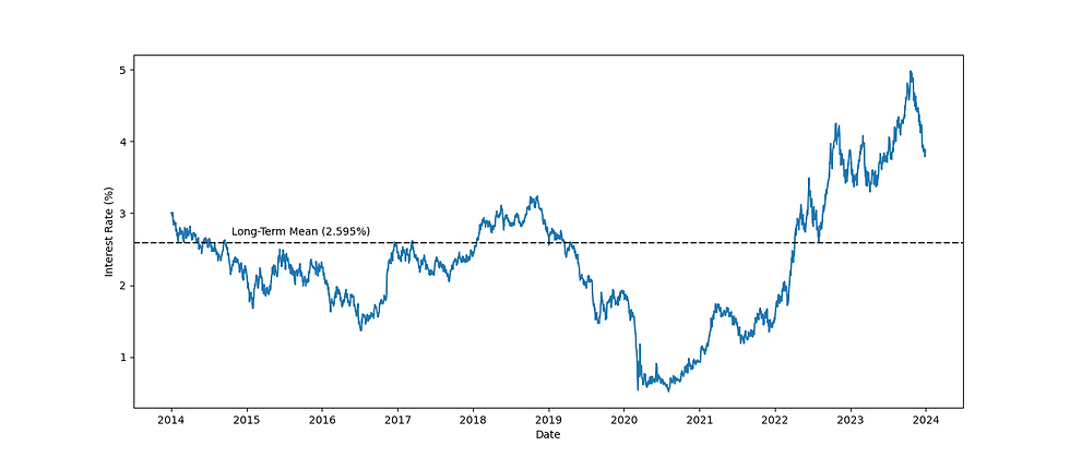
The figure visually confirms the mean-reverting behavior of rates and demonstrates how the Vasicek model captures the central tendency of interest rate movements over time.

• Long-Term Mean (𝜇): The calibrated long-term mean of 0.03901 suggests that, over time, the interest rate is expected to revert toward this level. This is slightly higher than the initial guess of 0.03456, reflecting the interest rate environment that prevailed during the 2022–23 period. The increase in the long-term mean is consistent with market expectations of tighter monetary policy during this timeframe.

  
  

• Mean Reversion Speed (𝛼): The calibrated mean reversion speed of 0.01013 remains low, indicating a slow reversion process. This suggests that while the rate tends toward the long-term mean, the adjustment occurs gradually—a behavior consistent with the observed relative stability in interest rate movements during the calibration window. It highlights the persistence of rate levels once they deviate from the mean.

  
  

• Volatility (𝜎): The calibrated volatility of 0.000758 confirms a low level of fluctuation in the short-term interest rate series. This is in line with the modest variability observed in the USD rate over the 2022–23 period, possibly due to economic factors or central bank policies aimed at controlling interest rate swings—thereby supporting a stable rate environment.

Evaluation of Calibration Performance

To assess the accuracy of the calibrated model, we compute three standard performance metrics:

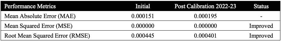
The Mean Absolute Error (MSE) and Root Mean Squared Error (RMSE) show improved accuracy post-calibration. The reduction in RMSE is particularly notable, indicating better overall alignment between model predictions and actual interest rate observations. These results demonstrate that the MLE-based calibration has effectively enhanced the model’s predictive performance.

Parameter Stability and Sensitivity Across Time Horizons

To assess the robustness and stability of the Vasicek model’s parameters, a similar calibration can be performed under two broader historical windows: 3 years (2021–2023) and 10 years (2014–2023).

The intention is to understand how the key parameters behave over slightly different time horizons, which helps in evaluating the robustness of the model. Comparing the calibrated values from 2022-23, 2021-23 and 2014-23 provides insights into the sensitivity of the Vasicek model's parameters to changes in market conditions, allowing us to evaluate whether the Vasicek model maintains predictive consistency or if its parameters exhibit instability when exposed to different economic regimes.

The table below shows the results of the calibration around different time frames, offering a comparative view of how these parameters adjust to reflect the interest rate dynamics over each respective period.

These results reflect how the Vasicek model adjusts its internal parameters to capture interest rate dynamics over different time frames.

The figure below presents the time series of the USD rate alongside the calibrated long-term mean.

The figure visually confirms the mean-reverting behavior of rates and demonstrates how the Vasicek model captures the central tendency of interest rate movements over time.

• Long-Term Mean (𝜇): The long-term mean increases from 0.02595 (2014–23) to 0.04160 (2021–23), before settling at 0.03901 (2022–23). This pattern reflects the upward shift in interest rate expectations as the market moved from a prolonged low-rate environment into a regime of monetary tightening (rate hikes) during 2022–23. The long-term mean appears reasonably sensitive to structural shifts, making it a valuable indicator of broader economic sentiment over time.

  
  

• Mean Reversion Speed (𝛼): There is a significant decline in the reversion speed as the historical window expands. From 0.0101 in the 2-year window, it falls to 0.00286 over 3 years and further to 0.00124 over 10 years. This trend indicates that the mean-reversion effect weakens when accounting for longer-term economic trends—especially in an era shaped by persistent low rates and unconventional central bank interventions.

  
  

• Volatility (𝜎): Volatility decreases consistently with longer calibration windows, from 0.000758 in the 2-year to 0.000522 across 10 years. This suggests that interest rate movements appear more volatile recently, whereas long-term trends are smoother, possibly due to the averaging out of short-lived fluctuations.

Implications of Extended Calibration

While the model successfully adapts to different historical environments, extended calibration also highlights its limitations in capturing short-term dynamics. Notably, the Root Mean Squared Error (RMSE) worsens slightly from 0.000401 (2-year window) to 0.000416 (10-year window), reflecting a decline in short-term predictive accuracy.

This decline is understandable, given the structural disruptions and unconventional policy regimes that shaped the 2018–2023 period. Factors such as near-zero interest rates, aggressive quantitative easing, and the economic shock from the COVID-19 pandemic, may have contributed to prolonged periods of low interest rates and delayed the return of interest rates to their theoretical long-term mean. As a result, the model’s ability to capture short-term market movements and extreme conditions is constrained when fitted across broad and diverse economic periods, impacting its overall accuracy and the alignment of predicted interest rates with observed market trends during this challenging period.

This calibration requires further analysis in this series, where the Vasicek model will be backtested against different interest rate environments, including extreme scenarios, to evaluate its robustness and applicability in interest rate risk management.