
How exactly does diversification help in reducing your portfolio risk?
In portfolio investing - we often hear the phrase, "don’t put all your eggs in one basket". If such a basket fails to hold your eggs then you may end up losing all your money. Similarly, if the invested funds are so concentrated in one investment asset and such investment fails, you will lose all your capital.
Diversification allows investors to allocate funds between different assets which helps in reducing the risk. Such diversification could be done between different asset classes or between securities within those asset classes. Diversified portfolios have a lower risk (measured by variance or standard deviation) than any other un-diversified portfolio or risk of individual asset position within that portfolio. This is due to the relationship that exists between different assets (called correlation) such that the overall risk is lowered by including additional assets in the portfolio.
The composition within the portfolio matters because each asset in a portfolio has its risk-return profile. By combining these assets, we can produce a risk and return profile for the portfolio itself. Different portfolios can be constructed by giving different weights to allocate the funds. We can then determine the portfolio composition that results in the best risk-return profile.
Let us understand how to construct an optimal portfolio feeding actual market data-
Let's consider a portfolio of five stocks- HDFC BANK, SBI, ICICI BANK, INDUSIND BANK & AXIS BANK with an exposure of $5million.
Extracted 737-Days closing stock prices of the period 01-01-2017 to 31-12-2019 from Yahoo Finance to calculate the daily continuous return (i.e., LN ( Sn / Sn-1 ) and deviation from its mean return (i.e., Return - Mean Return) for all the five stocks as shown below-
[ objective is to feed these returns and deviations into the solver to calculate the Expected Mean Returns and Standard Deviations for all the five stocks and use the same to construct an optimally diversified portfolio to maximize the overall portfolio return while keeping the risk minimum. ]
Step - 01: Calculate the Returns using Closing Stock Prices-
Daily Return = LN ( Sn / Sn-1 )

Step - 02: Calculate Expected Mean Returns and Standard Deviations for individual stocks-
Expected Return (μ) = SUM ( Return * Probability )
Excel Function =AVERAGE(returns range)Where,
Probability = 1 / no. of observations = 1 / n
Therefore,
Expected Returns are as follows-
HDFC Bank = AVERAGE(returns range) = 0.1024%
SBI Bank = AVERAGE(returns range) = 0.0428%
ICICI Bank = AVERAGE(returns range) = 0.1163%
IndusInd Bank = AVERAGE(returns range) = 0.0446%
AXIS Bank = AVERAGE(returns range) = 0.0708%
Standard Deviation (σ) = √SUM (Return - Mean Return) / n - 1
Excel Function =STDEV.S(returns range)Where,
Expected Return (μ) = SUM ( return x probability ) -- calculated already.
Therefore,
Standard Deviations are as follows-
HDFC Bank = STDEV.S(returns range) = 1.0457%
SBI Bank = STDEV.S(returns range) = 2.1068%
ICICI Bank = STDEV.S(returns range) = 1.8238%
IndusInd Bank = STDEV.S(returns range) = 1.8459%
AXIS Bank = STDEV.S(returns range) = 1.7581%
Step - 03: Calculate Expected Mean Return and Standard Deviation of the overall portfolio-
To calculate the expected mean return and standard deviation of the overall portfolio, it is important to decide upon the individual weights given to each stock in a portfolio.
At this point, it is better to understand the two critical aspects while constructing a portfolio-
The expected mean return of a portfolio is the simple average of the expected mean return of individual stocks but the standard deviation of a portfolio is less than the simple average of the standard deviations of individual stocks. This is due to the risk reduction benefit arising out of diversification, measured by the correlation coefficient.
The expected mean return can be extrapolated by multiplying the time period (say, 30-Day Return = 1-Day Return * 30) but the standard deviation is extrapolated by multiplying the square root of the time period (say, 30-Day Standard Deviation = 1-Day Standard Deviation * √30).
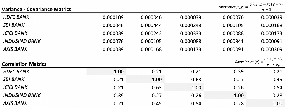
Please refer to Introduction to Covariance & Correlation - which explained in detail how to calculate the correlation coefficient. The outcome has been illustrated below-
If more weight is given to stock having a higher expected return, it will increase the overall expected return of the portfolio, and if more weight is given to stock having a higher standard deviation, it will increase the overall standard deviation of the portfolio. We know that to construct an optimal portfolio, we have to maximize the overall portfolio return while keeping the standard deviation minimum, and therefore, we got to use an optimizer engine (solver functionality in excel or a simulator in python).
The approach could be to maximize the expected return and minimize the standard deviation of the portfolio (just use random weights to proceed because the solver will automatically change/churn the weights by considering the target of maximizing the expected return and minimizing the standard deviation of the portfolio). Or, another approach is to calculate the Sharpe Ratio of the overall portfolio (being parsimonious) (a ratio that involves expected return, risk-free interest rate, and standard deviation of the portfolio -- excess return per unit of risk -- obviously, higher the better) and maximize the same. And this approach could be more simple because only one target is "to maximize the shape ratio".
Sharpe Ratio = ( Expected Return - Risk-free Interest Rate ) / Standard Deviation
Where,
1-Day Risk-free Interest Rate = 0%
Therefore,
Sharpe Ratios are as follows-
HDFC Bank = ( 0.1024 - 0 ) / 1.0457 = 0.0980
SBI Bank = ( 0.0428 - 0 ) / 2.1068 = 0.0203
ICICI Bank = ( 0.1163 - 0 ) / 1.8238 = 0.0637
IndusInd Bank = ( 0.0446 - 0 ) / 1.8459 = 0.0242
AXIS Bank = ( 0.0708 - 0 ) / 1.7581 = 0.0403
To calculate the expected mean return, standard deviation, and the sharpe ratio of our hypothetical-random-weighted portfolio (later be used as a seed to run the optimizer).

=SUMPRODUCT(individual weights, individual expected returns)

=SQRT(MMULT(MMULT(TRANSPOSE(portfolio weights), variance-covariance matrix), portfolio weights))
Portfolio Expected Mean Return (μp) = 0.0754%
Portfolio Standard Deviation (σp) = 1.2121%
Sharpe Ratio of the Portfolio = ( 0.0754 - 0 ) / 1.2121 = 0.0622
The outcome of the equally-weighted portfolio, maximum return at lowest risk portfolio, minimum risk at highest return portfolio, and the optimized portfolio has been illustrated below-

The Sharpe Ratio of the optimally diversified portfolio is the highest as compared to the other portfolios constructed and shown in the illustration above. The Standard Deviation (Risk) of our optimally diversified portfolio is the lowest as compared to any other portfolio or to any individual stock.

Drawbacks of the Portfolio Approach
More diversification the better?
There is no doubt that diversification helps in reducing the overall portfolio risk but,
diversification not only results in reducing the overall portfolio risk but after a certain point, it starts reducing the return possibilities as well and which can result in over-diversification. It occurs when the number of investment assets in a portfolio exceeds the level where the marginal loss of expected return is greater than the marginal gain of reduced risk. This pitfall in portfolio management actually erodes investor returns. Experts believe that a well-diversified or an optimal portfolio should comprise assets between 15 to 30 (spread across different asset classes, sectors, and industries) to diversify away, the unsystematic risk.
Please refer to Risk Mapping or Risk Decomposition - which explained how to manage risk if the number of assets in a portfolio is huge.
Opmerkingen