"What could be the maximum loss that can occur on my investments?"
[🤔] every investor would be thinking at some point in time.
Value at risk is a measurement tool used to assess the financial risk of an investment. It is one of the most widely used in addition to variance and standard deviation as it assesses the potential loss at a probability at which such loss will occur in a certain time frame.
In the early 1990s, J. P. Morgan developed an internal value-at-risk system that use to capture several underlying key risk factors in their portfolios, and the variance-covariance matrix was calculated using historical time-series data to compute value-at-risk numbers. These numbers were then aggregated to compute the overall portfolio's value-at-risk considering the correlations that exist between key risk factors.
Later, the value-at-risk measure became popular and globally adopted for measuring financial risk in trading portfolios. During these many years, many developments to this measure have happened to trade with the issues at various estimation points and many advancements have taken place to capture different types of financial risks and overcome the limitation of the VaR measure.

In a general context, the value-at-risk measure targets to calculate the maximum possible loss that can occur on an investment under normal circumstances at a certain confidence level in a given time frame. Most interestingly, this measure can be applied to a single position, on a portfolio of securities, or on an entire trading desk.
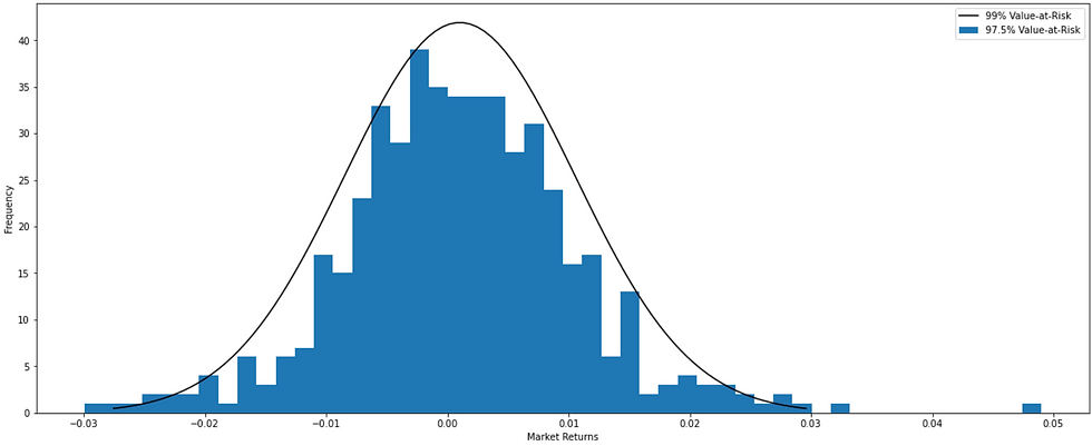
"under normal circumstances" - value-at-risk to be calculated under normal market conditions and for that, the calculated returns using the historical time-series data assumed to be normally distributed.

"a probability distribution is assumed to be normal if there are high probabilities that the estimated variable will result close to its mean and low probabilities that the estimated variable will result far from its mean of the distribution."

"at a certain confidence level" - value-at-risk can be calculated at a 95%, 97.5%, or 99% confidence level. The confidence level determines at what level the firm is willing to assess the risk.
"higher the confidence level, higher will be the value-at-risk number, and therefore, higher will be the certainty that the losses will be within the calculated value-at-risk"


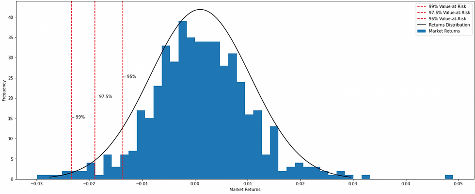
One has to increase the confidence level to dig into the tail of the return distribution to capture the extreme losses. Calculating value-at-risk at 99% will be considered to be a more conservative approach as that will capture more information regarding the nature of the tail return distribution; certain properties that 99% VaR can reveal but 95% VaR cannot.
Therefore, 99% VaR (-2.3430%) is greater than 97.5% VaR (-1.8926%) is greater than 95% VaR (-1.3676%) in terms of worst loss.
"in a given time frame" - the risk can be assessed at different time frames, also called value-at-risk horizon. This horizon refers to the period between two data points and that period could be 1 day, 10 days, 1 month, 3 months, or a year to calculate 1-Day VaR, 10-Days VaR, 1-Month VaR, 3-Months VaR, or 1-Year VaR respectively.
One also needs to decide upon how long would be the lookback period, the period for which such historical time-series data of all the risk factors needs to be extracted and applied to the risk model. Whether that period should be longer or shorter?
Statistical precision suggests;
a longer period to capture all the possibilities/events that have happened in the past.
a shorter period if non-stationarity and regime-switching are the key concerns.
from the regulators' standpoint, this period should be at least 252 trading days i.e. the time-series data on which this risk measure is based should capture all the relevant market changes over 252 trading days to date.
Once the historical time-series data is available and the model inputs are identified, one has to choose between the methods that can be used to calculate the value-at-risk number. The popular methods are (1). Historical Simulation Method, (2). Parametric Method (also known as Analytical Method), and (3). Monte-Carlo Simulation Method.
These methods used for calculating value-at-risk produce different results and there is no precise model for calculating the value-at-risk as these models come with their advantages and limitations but that is the next topic of our financial book.
The resultant value from the model will represent the value-at-risk number.
Suppose, if a portfolio of securities has a 1-Day 99% relative VaR of -2.3430%, it means that there is a 99% probability that the maximum loss on this portfolio could be -2.3430% over a single-day period with a 1% probability of its being exceeded. Therefore, the absolute VaR will be -2.3430% of $5 million = $-0.11715 million.
Limitations of Value-at-Risk (VaR):
It though has some valid reasons for its popularity, especially within investment banks and other big financial institutions, but it comes with a few limitations. Understanding these limitations is crucial for effective risk management, especially in periods of market stress.
Dependence on Historical Data: VaR calculations rely heavily on historical data to predict future risks. If the historical data does not include extreme market conditions, the VaR estimates may be too optimistic.
Lookback Periods: The lookback period, or the timeframe of historical data used, can significantly impact VaR calculations. If the lookback period is too short or does not capture periods of market stress, the VaR will not accurately reflect potential extreme losses.
Market Stress: VaR does not account for potential losses during periods of extreme market stress not captured in the lookback period. This limitation became evident during the 2008 financial crisis when many portfolios experienced losses far exceeding their normal VaR estimates. for example: during the 2008 financial crisis, market conditions were much more volatile and severe than in previous years. Many financial institutions relied on VaR models that did not account for such extreme scenarios, leading to underestimation of risk and significant financial losses.
Correlation: When it comes to determining the risk of a portfolio, a risk measure is expected to incorporate the correlation between each pair of assets. However, with the increased number of assets and diversity of positions in the portfolio, it becomes very difficult to calculate and incorporate the correlations precisely for risk reduction.
Non-Additive Measure: Speaking about the first limitation, this risk measure becomes non-additive. "the value-at-risk of asset A plus the value-at-risk of asset B is not equal to the value-at-risk of a portfolio containing asset A and B due to the correlation that exists between them."
VaR Method Selection: As mentioned earlier, one has to choose between the methods that can be used to calculate the value-at-risk number. However, different methods eventually lead to different results. It becomes difficult to make the right choice between these methods: The Historical Simulation Method, Parametric Method, and Monte-Carlo Simulation Method.
Beyond VaR: Value-at-Risk does not measure the worst-case loss i.e. unexpected loss beyond the confidence level. 99% 1-Day VaR means that in the remaining 1% of the cases, the losses are expected to be greater than that 99% 1-Day VaR number. This measure does not say anything about the severity of the losses within that 1% case.

Comments